Download Now
O'Reilly's Book "Building ML Systems" First Chapter Available!


Training an ML model nowadays is the easy part — managing the lifecycle of the experiments and the model is where things get complicated. Luckily, Weights and Biases provide the developer tools that with a couple of lines of code let you keep track of hyperparameters, system metrics, and outputs so you can compare experiments, and easily share your findings with colleagues. However, the value of the model comes from operationalizing and turning the model into a prediction service. This requires making data available to these services consistently to how the models were trained. Hopsworks 3.0 introduced a new Feature View abstraction and now supports KServe for model serving. Together these two features provide the APIs to consume data from the feature store consistently between training and production and allow you to deploy models from your Weights and Biases model registry into production quickly, providing a Rest Endpoint to perform prediction requests against.
MLOps has become a common term in the machine learning space, however, it is often misunderstood. When we talk to customers and users, many practitioners assume MLOps is the practice of adding a structured process with CI/CD to model development using tracking technologies like Weights and Biases (W&B). W&B aims to provide the tools to build better models faster with experiment tracking, dataset versioning, and model management. While producing better models using a structured development process is desirable, nevertheless, if you look more closely, the actual bottleneck of MLOps is the deployment of a ML model such that it can reliably and efficiently produce predictions to support enterprise decisions.
In practice, this means enterprises need infrastructure to run a prediction service on. There are two ways to build a prediction service that uses a model to make intelligent decisions:
As we add infrastructure to the mix, the concept of MLOps suddenly becomes much harder, and it shows in a recent survey, which found that only 11% of organizations succeed in putting models into production in less than one week:

In this blog post we will describe how you can easily make the journey from ML models to putting prediction services in production by choosing best-of-breed technologies, W&B for development, and Hopsworks as a feature store and serving infrastructure.
The value of ML models is realized either when (1) predictions are made on a regular basis, and then fed back into operational systems (e.g., Salesforce for CRM) where the business can act on the predictions and in some form improve decision making or (2) when a user/customer interacts with a product which is powered by an online ML model improving customer experience.
As mentioned above, predictions can be made in two ways, in batches and online in real-time. Both have different requirements, but in order for them to produce a new prediction, they need access to new data, which means they need to be connected to one or more feature pipelines. A feature pipeline is like a data pipeline, except it produces features as output (instead of curated datasets prepared for efficient querying).
If you write feature pipelines without a feature store, typically, each model gets fed by one feature pipeline - even if some of the features created are needed by different models in production. That is, there are multiple different implementations of the same features that can lead to inconsistencies in their implementation and it also creates inefficiencies in terms of duplicated work. This is one of the reasons why operationalizing models takes so much time, because this work has to be repeated for every new model. Additionally, the same feature pipeline is probably also used for model training, leading to additional complexity, as the feature pipeline for inference and the feature pipeline for training need to be kept consistent.

For batch applications you can get quite far by using an execution engine, like Apache Spark, an orchestration framework like Apache Airflow, and object storage like S3. For real-time predictions, the latency requirements are different though, and you cannot run the feature pipeline synchronously before the prediction, as it would often add too much latency to the prediction request. So you need to store the pre-computed features somewhere where they are accessible at low latency - an online feature store.
Additionally, you need the infrastructure to provide a network interface, like REST or gRPC, to the model, so you can send a primary key value to the endpoint, which will then in turn look up the correct corresponding features, pass them to the model and return the prediction.
This leads to two requirements to address:
The Hopsworks Feature Store is addressing the first requirement. It provides a central funnel for all features to be used in production. With its dual database architecture, it can serve both real-time as well as batch inference and training data. Instead of having a feature pipeline for each feature-model combination, we only have a pipeline for each feature, feeding into the feature store. We provide a Feature View API, that lets developers reuse features across models without any data copying.
To address the second requirement, Hopsworks now supports KServe for model serving, with new low latency access to model deployments using Istio. We also introduce a new Python SDK for managing models and deployments.

Before we can move to the deployment of a model, we need to train a good machine learning model. The model development process tends to produce a lot of metadata and artifacts, which is valuable to capture in order to develop strategies to improve model performance, but also for the debugging of models and tracking their lineage and dependencies.
For this purpose, Weights and Biases provide a platform to track all of the information and artifacts produced when training models and experimenting with models. Weights & Biases (WandB) provides 5 main functionalities:

W&B is easy to use, provides a full model registry and is very popular among Data Scientists, since it enables them to train better models and share them easily within teams and organizations.
However, W&B does not directly help you with the two requirements that we defined in the previous paragraph. W&B does not provide serving infrastructure for the model nor for the features. Therefore, it’s the perfect complement for Hopsworks.

Hopsworks Feature Store comes with two main abstractions: Feature Groups and Feature Views, which provide the API for writing to the feature store and access to the feature data. Feature groups are tables of features that are either stored in Hopsworks as Hudi tables or external (virtual) tables from Data Warehouses, like Snowflake, Redshift, and others.
Feature Views are logical groups of features that provide an API to read features from the feature store. Hence, as a W&B user you will mostly be a Data Scientist looking to train a model and therefore you will in most cases end up using the Feature View API.
At a high level Feature Views represent the set of features needed by a given model. While Feature Groups store the feature data (e.g., the output of an aggregation). Features in Feature Groups are typically stored as untransformed features (not normalized, one-hot encoded, etc). The main motivation for storing untransformed features is that they are easier to reuse than transformed features. If you store only fully baked (and transformed) features, you can only train models on all of the feature data in a feature group. Otherwise the transformations already applied to those features might be incorrect on the subset of feature data you want to use for training (e.g., if a numerical feature was normalized using its arithmetic mean computed over all data, and you want to use a subset of the features, the arithmetic mean may be different for your subset, and the features incorrectly transformed). This is particularly true for seasonal and time-series data.
So, we should store untransformed features in feature groups to maximize reuse. Different models can then apply different transformation functions to different features over different ranges of feature data. Transformation functions should be applied on-demand when the features are read - as training data or inference data - using the Feature View. The Feature View stores metadata about which transformation functions are applied to which features and the statistics of the training data to be used for the transformation (e.g. arithmetic mean and standard deviation). Data scientists can then use Feature Views to generate training data, potentially over different time windows.
The same Feature View can then be used by analytical models to generate batch data for inference - and by operational models to generate feature vectors for real time predictions. The Feature View will ensure the consistency of both the schema and transformations being applied between model training, batch inference, and real time predictions.
Creating a Feature View from features in the Feature Groups: trans_fg and window_aggs_fg
Once the feature view is created, users can easily use it for the following four operations:
Examples of using the Feature View APIs
In the above code snippet, we show (lines 2-7) how to create training data in csv file(s), (line 10) retrieving training data as train/val/test sets in Pandas DataFrames, (lines 13-15) retrieving batch inference data for a given time range, and (lines 18-19) retrieving a feature vector as a Python array that will be sent to the online model for inference.
Once you have trained your model and you have it saved as an artifact in W&B, we can deploy it to Hopsworks. We will show here how to deploy it as an online model, however, the same applies to a batch model, instead of a predictor script you will have a batch-inference job that could be run in Python or Spark on any platform (including Hopsworks).
In order to make Hopsworks aware of the model that corresponds to a feature view, we can use the concept of Tags in Hopsworks:
Link your final WandB model to the feature view with a tag
The tag should contain all the information needed in order to download the needed artifacts from W&B.
We can then connect also to W&B to download the artifacts and register them on Hopsworks.
Download the model artifacts from WandB
In addition to the model artifact, we need an instance of a predictor class that implements the predict API in order to tie together the model and the feature store:
Prepare the predictor script
As you can see the script initializes the feature view for online serving, and then every request to the model’s network endpoint will invoke the predict method, retrieving the precomputed features from the feature store, and passing them to the model for prediction. The predictor script will look exactly the same in most cases apart from the feature view name and version to be used. Hence, if you have your W&B project version controlled and pushed to GitHub, you can also keep a template of the predictor script in the same repository. Using CI/CD it is then possible to easily template the predictor script, replacing the feature view name and version when a new model should be deployed into production. This way you can automate the steps shown in the next code snippet.
With these two things in place we can deploy the model to Hopsworks, by first registering the artifact and then deploying the predictor script:
Deploy the model
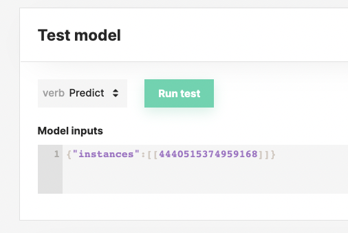
You can now test the model by sending REST calls or simply through the UI:
Congratulations. You now know how to build an operational model using W&B and Hopsworks. Get started for real with our W&B tutorial notebook together with serverless Hopsworks on hopsworks.ai.


© Hopsworks 2024. All rights reserved. Various trademarks held by their respective owners.