The Journey from Star Schema to Snowflake Schema in the Feature Store
Add more features to your ML model with a Snowflake Schema
In this article we introduce the snowflake schema data model for feature stores, and show how it helps you include more features to make better predictions
This article is part 3 in a 7 part series describing in lay terms concepts and results from a SIGMOD 2024 research paper on the Hopsworks Feature Store.
Other Parts: 1 (Modular/Composable AI Systems) , 2 (The Taxonomy for Data Transformations), 4 (Lakehouse for AI), 5 (From Lakehouse to AI Lakehouse), 6 (Real-Time AI Database), 7 (Reproducible Data).
More Features makes for Better Predictions
Mary is building a real-time credit card fraud prediction model that has a strict 50ms latency SLO (service level objective). Every credit card payment arrives at a server with minimal information - the credit card number, transaction amount, longitude and latitude of where the translation took place, and whether it was online in the real-world at a merchant point of payment. That information is not sufficient to train a high performance machine learning (ML) model to predict whether the incoming transaction is fraudulent or not. She learns that feature stores can provide her with low latency access to precomputed features that could enable her to have a rich enough model to perform good enough for fraud detection. The credit card transactions land in a Kafka cluster and a streaming feature pipeline can be used to compute aggregated usage statistics over windows of time (last 15 mins, hour, day, week). Anomalous patterns of credit card usage can be detected by the model - great. She could also use the location of the current credit card transaction and the location of the previous transaction to compute a feature that is predictive of a geographic attack - for example, if the card is used in Paris, then 1 hour later in New York.
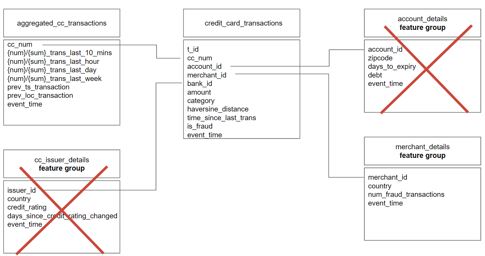
Figure 1: Mary can’t use the cc_issuer_details or account_details features as the credit card transaction as her feature store only supports a star schema data model. The credit card transaction does not include primary keys for the cc_issuer_details or account_details, and it would introduce too much latency to resolve them from the existing operational database, so she doesn’t use those features in her fraud model.
Mary does some offline experiments that show that there are features related to the account holder and the credit card issuer (recently, there has been an increase in single use virtual credit cards) that would further help improve the accuracy of her model. However, she encounters a problem. Existing feature stores only support a star schema data model. That means, when the credit card transaction arrives at the online model, she needs to provide the primary keys for all features that are retrieved from the feature store. That was easy for credit card features (and merchant features, when the merchant identifier is included with the transaction) as she could use the credit card number to retrieve the precomputed features. The transaction did not include, however, an identifier for the card issuer or the account holder. She considered making calls to retrieve these 2 IDs using primary key lookups on two different tables in a Postgres database. However, operations were not happy about opening access to their production database and the ~15ms p95 latency would have blown her SLO budget. So, she just went to production without the card issuer and account holder features. Not her fault.
So, how could Mary have included the card issuer and account holder features? If her feature store supported a Snowflake Schema (nested tables), not just a star schema, she could have retrieved all.
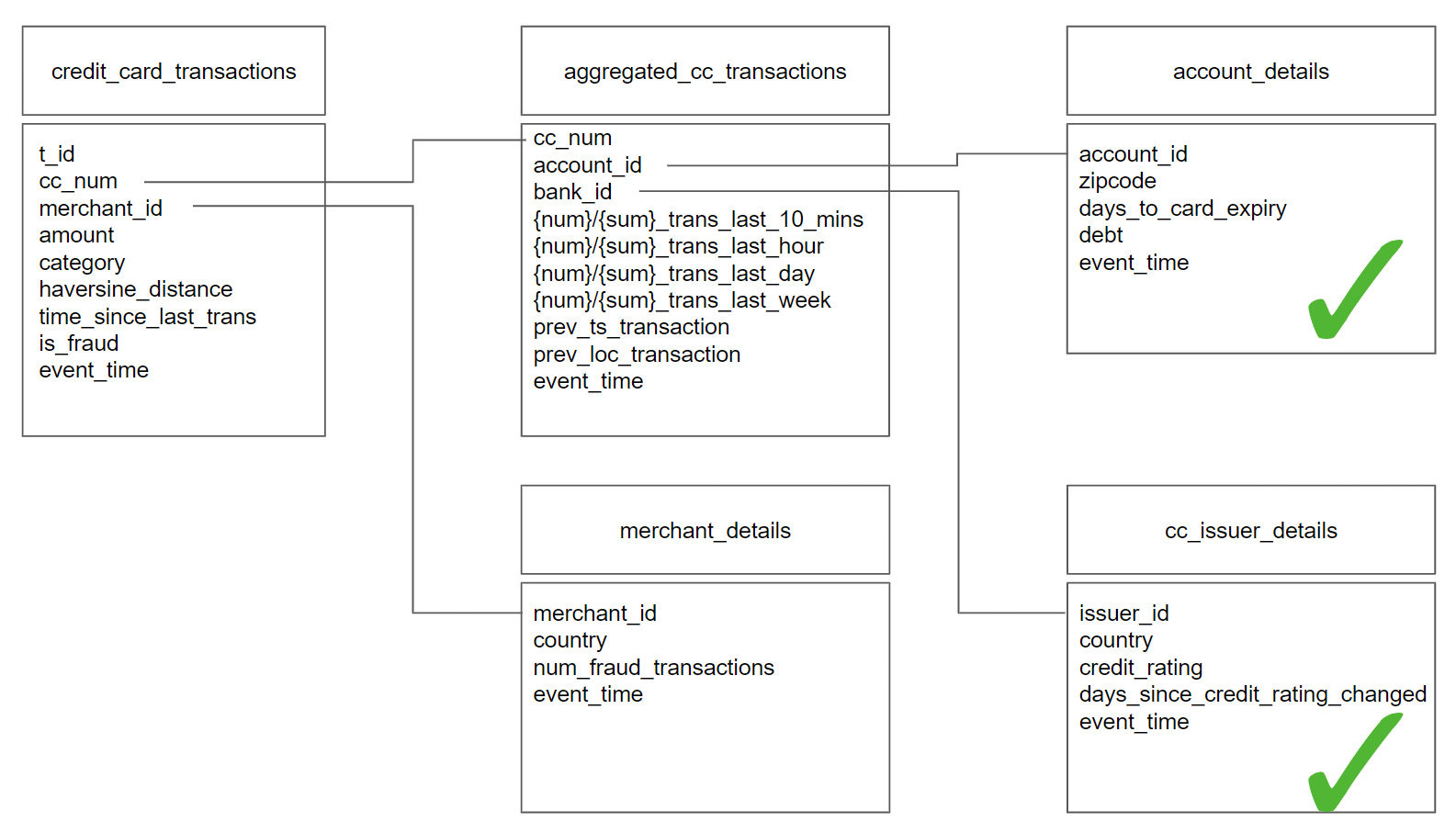
Figure 2: Mary can now use the cc_issuer_details and account_details features as her feature store supports the Snowflake Schema data model. This enables her to read these features in nested tables in a single pushdown LEFT JOIN query.
Snowflake Schema in Hopsworks
In Hopsworks, we call tables of features feature groups. Feature pipelines are programs (in Pandas, Polars, SQL, Spark, Flink, Feldera, Bytewax, Quix, etc) that periodically (or continually for streaming feature pipelines) update the feature data stored in feature groups. Each feature group stores its historical feature data in a table format (Apache Hudi or Delta Lake) on object storage and its low latency feature data for online models in a table in RonDB. So, how do we define a data model in Hopsworks?
Each feature group in Hopsworks has one or more columns as its primary key (the entity identifier). The foreign keys (shown in figures 1 and 2) are just columns in a feature group (there are no foreign key constraints). When you want to create a model and select features from more than one feature group, you have to use our feature selection API. For the Star Schema data model from figure 1, the code looks like this:
Here, for every child of the credit_card_transactions table in the Star Schema, we call nested join methods. All tables are children of the parent credit_card_transactions table. We pass the selected features to a feature view in Hopsworks, that is later used to create training data and retrieve feature data for inference, ensuring no skew between training and inference.
In online inference, when you want to retrieve features in your online model, you have to provide all 4 foreign key values from the credit_card_transactions feature group to retrieve your precomputed feature values using the feature view.
For the Snowflake Schema data model from figure 1, the feature selection code looks as different, as we have to build up the subtrees:
First, we build the subtrees with nested tables (subtrees) using joins, and then we join the subtrees to their parents (the root credit_card_transactions node).
Now, we have the benefit, that in online inference, we only need to pass two foreign key values to retrieve the precomputed features:
Internally, Hopsworks will perform two parallel queries - a primary key lookup on the merchant table in RonDB, and a pushdown LEFT JOIN to retrieve the other features from the aggregated_cc_transactions, issuer_details, and account_details tables.
Pushdown Left Join Performance Analysis
RonDB implements a pushdown LEFT JOIN to reduce the latency in retrieving nested features from a Snowflake schema data model. Figure 3 shows how we implement pushdown LEFT JOINS in our online feature store database, RonDB.
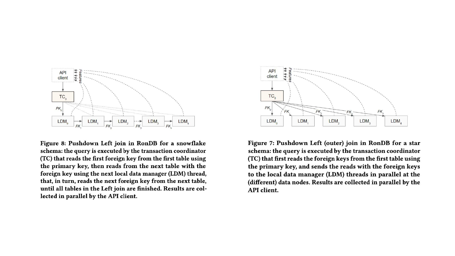
Figure 3: In our SIGMOD paper, we show how we implement the pushdown LEFT JOIN, where the nested foreign keys are iteratively resolved in the database nodes, instead of in the API client (which would lead to higher latency). Star schema features are resolved with parallel primary key lookups to the tables, while nested features are resolved with a pushdown LEFT JOIN.
The Hopsworks feature store client issues parallel queries for all features from different tables (feature groups) in RonDB. For child tables (star schema), a primary key lookup is used to retrieve features from RonDB, while nested features are retrieved by issuing a pushdown LEFT JOIN to RonDB. For wide tables, with many features, and where only a small number of features are required, RonDB supports projection pushdown. For example, if you have a feature group (table) with hundreds of features, but only need a few of them for the current model, RonDB will only read and return the data for those features. Many databases or key-value stores used as feature stores, most notably Redis, do not support projection pushdown. Without projection pushdown, the entire row is returned and the filtering is performed in the client. For rows of 10s or 100s of KB, this could mean 100s of times more data is transferred than needed, negatively impacting latency and throughput (and potentially also cost).
In Figure 4 below, we also see the performance improvement of pushing down the LEFT JOIN to the database.
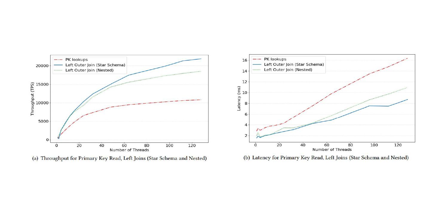
Figure 4: Pushdown LEFT JOINs reduce latency and improve throughput for feature stores.
We didn’t include any performance numbers in the paper for projection pushdown or predicate pushdown (both supported by RonDB), as these are not novel concepts in the database world - research papers favor novelty over known concepts. However, projection pushdown and predicate pushdown are must-have functionality for your feature store if you care about performance at scale.
Conclusions
This article explores the limitations of existing feature stores that only support Star Schema data models and introduces the Snowflake Schema data model, now supported by the Hopsworks Feature Store. The Snowflake Schema enhances online models by incorporating additional features through nested tables. In RonDB, we showed how the pushdown LEFT JOIN in RonDB reduces the latency and improves throughput for nested queries in Snowflake Schema data models.