Pandas2 and Polars for Feature Engineering
We review Python libraries, such as Pandas, Pandas2 and Polars, for Feature Engineering, evaluate their performance and explore how they power machine learning use cases.

Introduction
In the world of Data Science, Python is one of the most common terms you will come across. Python is a general-purpose programming language loved and cherished by Data Science professionals. It is easy to use and hosts many libraries and frameworks designed to handle data-related workloads. These libraries provide convenient functions that help with tasks like
- Data Ingestion
- Data Processing
- Feature Engineering
- Machine Learning Training
- Model Deployment
This blog will talk about using Python for Feature Engineering tasks. More specifically, we will discuss libraries, including Pandas2 and Polars, and their role in enabling easy feature engineering for machine learning use cases. Moreover, we will also conduct a comparative performance analysis to decide which framework suits better in what scenario. Before any of that, let’s start by understanding what Feature Engineering is.
What is Feature Engineering?
Feature engineering is a wide umbrella that encompasses various data processing techniques to generate new data from existing features. Features are the crucial information input to a machine learning model and help it understand patterns within data. The model learns to connect these features to the output values and make predictions in unseen scenarios. Features that can represent the output variable clearly are considered high-quality and help improve the model's performance.
However, in most practical cases, the features in default datasets are insufficient for the model's learning. Feature engineering also allows data scientists to extract better representations of the information from existing data through new features. These new features help the model perform better and save engineers from the hassle of additional data collection.
Common Feature Engineering Techniques
Feature engineering uses common mathematical and statistical functions on existing features to generate new values. Some common techniques include:
- SUM: Summing values across subsets of data is helpful in getting aggregated information. An example would be to sum total sales on a weekly basis.
- Average: Similar working to summation, but it would give the average of a value. Calculate the average price of a product sold over a few months.
- Count: Aggregate the data by getting the number of records against a subset of the data.
- Rolling Average: Create a running total for specific values. This feature provides granular aggregations based on a daily basis.
- Date Parsing: Dates are primarily presented in a combined format (dd/mm/yyyy etc.).
The values can be parsed and separated into
a. Day
b. Month
c. Year
d. Week
e. Day of Week
The individual values allow the model to emphasize each aspect of the data more.
These techniques are difficult to understand without practical demonstration. Let’s try to apply them in Python on a real-world dataset.
Feature Engineering Frameworks: Pandas, Polars and Pandas2
There is little benefit to discussing such techniques without viewing their practical applications. For this purpose, we will use the data processing frameworks hosted in Python. We will carry out similar processing in Pandas and Polars and then in Pandas2 (The latest release from Pandas). This section will see feature engineering in action and compare the frameworks in terms of performance.
Here are the systems specs used to carry out the data processing:
Processor: AMD Ryzen 5 3600 (6 core 12 Thread)
RAM: 16 GB
Disk: 1 TB SATA SSD
Note: For a fair comparison, all frameworks are tested on the same system, and the processing times presented are from the first run; this is important since some frameworks can cache commands for better performance in subsequent runs.
We will be using the Python notebook magic function `%%time` to evaluate the execution time of the commands, and the time comparisons will be mentioned in the next section. You can access the colab notebook here.
Pandas
First, we need to install the appropriate version of Pandas. Run the following command in the terminal.
Specifying the version number is important since the latest stable version is 2.0.3 at the time of writing. To test the conventional framework, we must use the older stable release.
Once installed, we can read our test dataset. The dataset we are using is the testing data from the TalkingData AdTracking Fraud Detection Challenge 2018. The dataset is 843 MB on disk. Let’s load it into memory.
Let’s see the shape of this dataset and take a look at the data present inside.
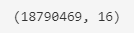
Figure 1: Shape of the dataset
Our dataset contains roughly 18 Million rows!
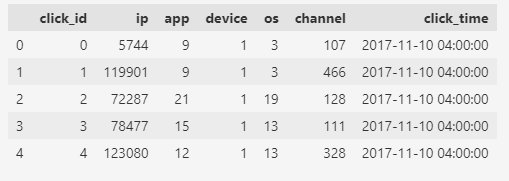
Figure 2: First 5 rows of the dataset
It is also helpful to get some insights about the data. Luckily Pandas has a function for that.
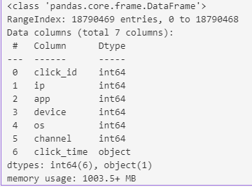
Figure 3: Dataset Info
Looks like our dataset is consuming a little over 1 gigabyte of memory. We also see that it contains 7 columns, all of which are inferred as int64 except for `click_time`, which is loaded as an object. Our first step will be to convert this into a datetime type.
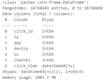
Figure 4: Datatypes after conversion
Data types are all set now. Let’s move on to performing date parsing. We will extract Year, Month, Day, Hour, Minute, and Second from the date column.
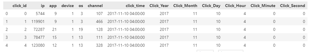
Figure 5: Dataset after date parsing
Now, it's time for some complex calculations. For further feature engineering, we will calculate the number of clicks an app gets on an advertisement per second, minute, and hour. This will require us to apply a `groupby` clause across the time features and count the number of occurrences against the app id. Then we will append the values back to the dataframe using the join operation. We will monitor the performance of all these actions combined to get a realistic view of how Pandas perform.
This operation concludes our feature engineering process. Let’s look at the final dataframe.
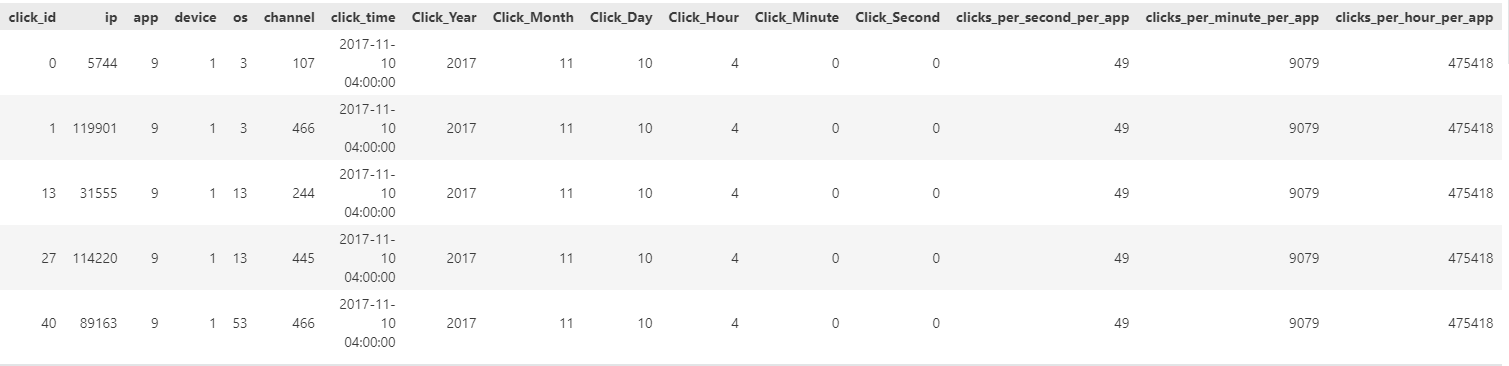
Figure 6: Final Dataset
We will now perform these same operations in Polars.
Polars
Polars is a new contender for Pandas. It is implemented in RUST and possesses amazing parallel processing caching capabilities which provides it with blazing fast performance. Now we will see how Polars compares to Pandas in the type of operations that we performed above. The first step would be to install the required framework.
Next, we will carry out the same procedures as in Pandas. Luckily many of the functions in Polars follow the same nomenclature as Pandas so the learning curve is not too steep for new users.
Reading data file.
Polars does not have any function to get information for the dataset, so we will use the `estimated_size` function to get the dataset size in memory.
The dataset, loaded in Polars, occupies a total of 1343.99 MB of space. Let's preview the dataset.
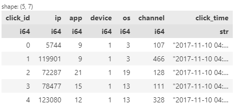
Figure 7: Dataset in Polars
Polars displays the dataframe in a similar fashion as Pandas and it also displays the data type for each column. The `click_time` is still interpreted here as a string so we will have to change that.
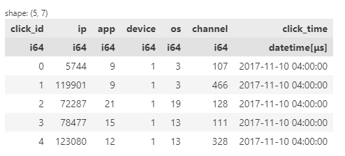
Figure 8: Dataset after datetime conversion
Now we will parse the date field into granular components.
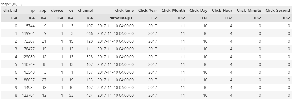
Figure 9: Dataset after date parsing
Now the last step remains to perform aggregations to get total clicks on a per second, per minute and per hour basis.
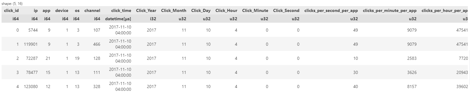
Figure 10: Dataset after all feature engineering procedures
That concludes our feature engineering code with Polars. The time comparisons have some very interesting results but we will discuss those in the Performance Review section. Now we will try out the new iteration of Pandas, i.e., Pandas2.
Pandas2: A New Challenger
Pandas2 was released earlier this year with the aim of offering a significant performance gain over its predecessor. The main change comes in the form of Apache Arrow which is used in Panda2 as a back-end. Arrow is designed to handle large-scale datasets and has added benefits like parallel processing and lazy evaluation.
Let’s begin by installing Pandas and Pyarrow in a new environment. Note that presently the default stable version for Pandas is greater than 2.0 but we will specify it just to be sure.
After the installation is complete you will notice that not much has changed. The library will be used in the exact same way as its predecessor. The only change will occur when setting the back-end.
Note that this time we have specified the engine as ‘pyarrow’ and the data types as Arrow dtypes. The syntax will remain exactly the same for the rest of the processing.
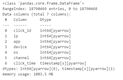
Figure 11: Dataset info with Pandas2
The data types are now in the pyarrow format and it has auto-detected the `click_time` column as a timestamp so that’s one step we can skip in this code. Since all the processing remains the same, the entire code is presented as a single code block below.
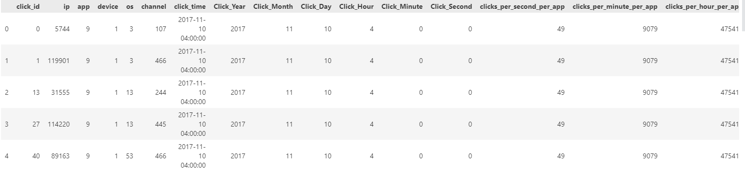
Figure 12: Final data set after Pandas2 processing
Performance Review
Each of the frameworks were evaluated against the time they took to perform the operations. The results are summarized below.
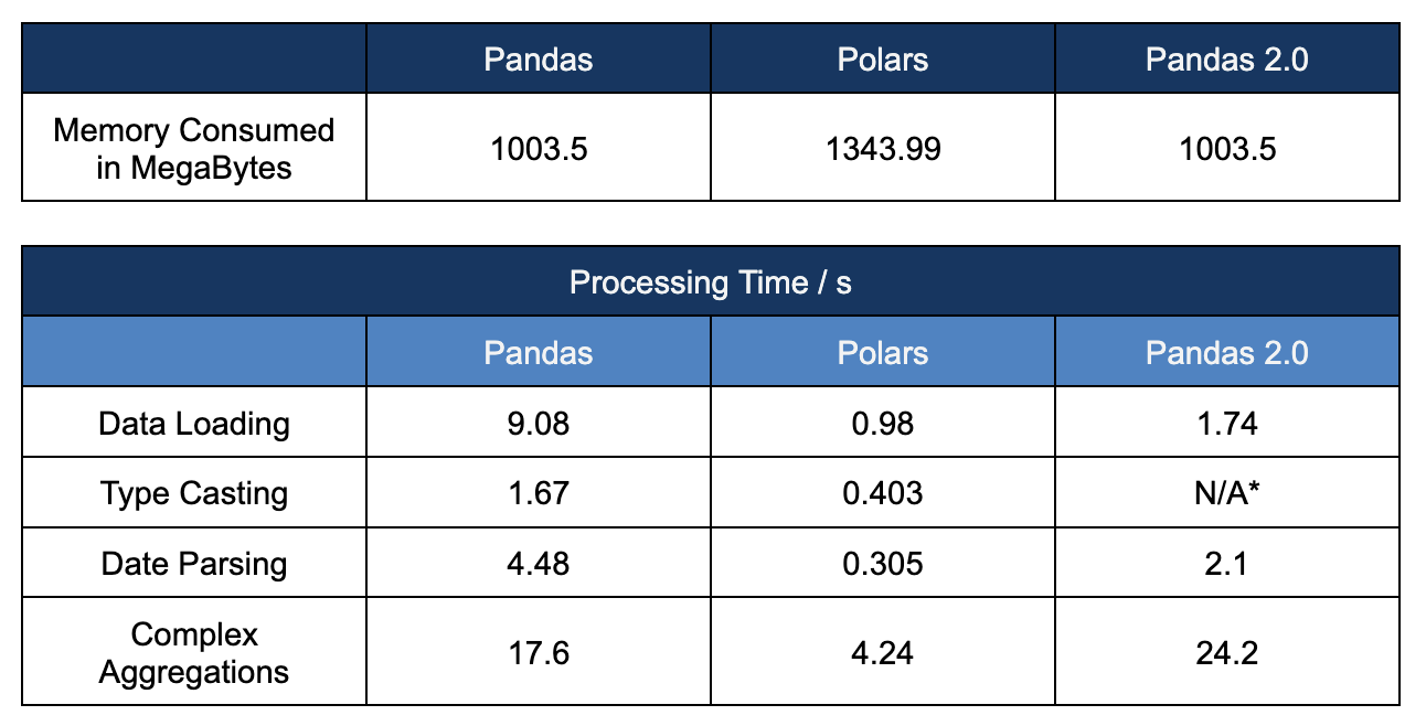
Figure 13: Summarized results of processing times
*type-casting was skipped with Pandas2 since the framework auto inferred the correct data type.
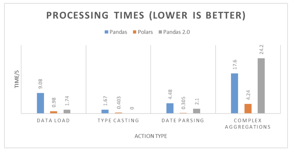
Figure 14: Processing times comparison
We have some interesting results in our hands. While Polars took a few extra Mega Bytes to store the data, it clearly outshines Pandas, with a performance gain of up to 10x, in every action we have performed. While Pandas2 does offer a performance gain over its older version, it seems like a hit-or-miss process. While it took less than half the time in our date parsing step, it showed worse performance compared to both its counterparts.
Which Should You Use?
The decision to use a specific data framework depends on the data type you are working with. We have already seen that Polars is a clear winner against Pandas in terms of performance. This is largely due to its ability to spread processing across various CPU cores. If you are working with a large-scale dataset spanning Gigabytes or even Terabytes, then Polars is a clear choice, especially since it is now stable enough. However, if you are used to Pandas and work with light data, there is no reason to switch since adjusting to something new would take time.
Pandas2, on the other hand, is a different story. While it does have some performance benefits over Pandas, the processing times are not consistent. Despite regular updates, Pandas2 is still under construction and should not be used for day-to-day professional work.
Writing Features to Hopsworks
The final step to a feature engineering pipeline is storing the features in a scalable, fault-tolerant feature store. Hopsworks feature store offers a simple API to store and access data features. Let’s store our engineered feature in a designated feature store.
The features can now be accessed using the same API whenever required and can be versioned over various iterations of the feature engineering pipeline.
Summary
A machine learning model’s performance depends on quality training features, which most real-world datasets lack. Feature engineering techniques allow data scientists to extract meaningful information from the available data and append it as additional features. Python includes various libraries that facilitate the feature engineering process. Pandas and Polars are popular frameworks that include various functions to ease data processing procedures and throughout this blog we have compared Pandas, Polars and Pandas2. While Pandas and Pandas2 are the go-to solutions for almost every data scientist, Polars is becoming increasingly popular due to its exceptional performance gain over the former. The last step to every successful feature engineering pipeline is storing the features in a suitable feature store such as Hopsworks. Hopsworks provides fault-tolerance and version control for your features and facilitates your machine-learning experimentation.