Feature Engineering with DBT for Data Warehouses
Read about the advantages of using DBT for data warehouses and how it's positioned as a preferred solution for many data analytics and engineering teams.

Introduction
Feature selection and feature engineering are crucial steps in any data science project. It is where we use raw variables to create meaningful relevant features for machine learning models. During the exploratory stage, we can create the features we want in a Jupyter Notebook or even scripts! However, businesses often deal with large and complex data so it could rapidly become a potential nightmare in terms of maintenance. We need tools and platforms to create and implement features pipeline in production efficiently. One such amazing tool is DBT(Data Build Tool).
Preparing data is not restricted to machine learning, analytics teams have also welcomed the arrival of DBT and many of them today consider it as the go to tool to build data preparation pipelines.
In this article you will be introduced to DBT, its advantages for data warehouses, and how you can use some of its features to build data transformation or feature engineering pipelines.
What is DBT?
DBT (Data Build Tool) is an open-source tool that enables data analysts and engineers to transform data in their data warehouse more effectively. It allows users to define transformations as SQL queries and manage dependencies between them. DBT compiles these queries and runs them in the appropriate order, ensuring that each step is built upon a correct and up-to-date foundation.
Understanding DBT and its Features
DBT is a powerful tool designed for data transformation and workflow management in data warehouses. Its key components are:
-
Models: They are the core of any DBT project. They represent SQL queries that transform raw data into a more useful state. They are stored as `.sql` files where each file corresponds to a single model. DBT compiles these models into executable SQL and runs them in the data warehouse of choice.
-
Snapshots: They are used for capturing historical data changes over time. They allow tracking of how rows in a table change, giving a view of the data at any point in history. Snapshots can be used for auditing, reporting, or analyzing trends over time.
-
Tests: The purpose is to ensure data integrity and accuracy.It can be custom SQL queries that DBT will execute to validate data against specified conditions (e.g., uniqueness, not null, referential integrity).Through tests, we can catch data issues early in the pipeline and save costs. Tests are automatically run by DBT after models are built.
-
Documentation: It is essential for maintaining clarity and understanding in projects. DBT allows for the documentation of models, their columns, and the project as a whole. It Uses a combination of Markdown and special schema YAML files.This Helps in making the data transformations transparent and understandable.
These components work together within DBT to create a robust, maintainable, and transparent data transformation workflow. By leveraging these elements, data teams can build scalable, reliable, and well-documented pipelines.
What are the Advantages of DBT for Data Warehouses?
DBT is particularly beneficial for several reasons:
-
Efficient Computation of KPIs and Aggregates: In many data-driven environments, there is a continuous need to compute Key Performance Indicators (KPIs) and aggregate metrics at various levels to feed into dashboards and reports. DBT efficiently handles these operations, ensuring that the data is accurate and updated.
-
Handling Complex Data Pipelines with Lineage: DBT helps manage complex data pipelines by maintaining data lineage, which is crucial for understanding how data transforms through various stages and impacts the final output.
-
Integrated Scheduling: With DBT, there is an integrated scheduling feature that automates the transformation processes. This means that data engineers can set up schedules for data transformation tasks, ensuring that the latest data is always available for analysis and feature engineering.
-
Scalability and Robustness: DBT offers the tools required to transform data effectively. When combined with a scalable data warehouse (for instance: Redshift, BigQuery..) it allows for the creation of robust, insightful features that can be used to build highly accurate predictive ML models.
Finally, here is a summary of the advantages that this tool offers:
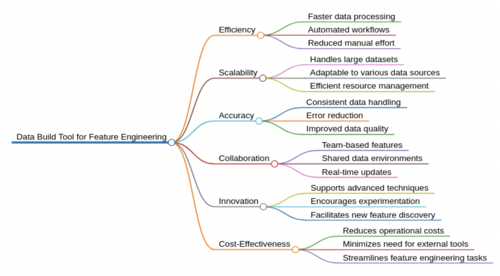
Figure 1: Benefits of Utilizing DBT for Data Transformation
Now let’s dive through some practical examples, to run them we used a dbt cloud connected to an AWS redshift warehouse. The preparation of the redshift cluster is out of scope of this article, you can get more insight into how to do it by visiting the aws documentation.
Feature Engineering with DBT
As far as DBT is concerned, we can either use:
- A managed solution (dbt cloud)
- A self hosted one that could be installed within our local environment.
For this article we will use DBT cloud and a sales table that could be downloaded here (transactions table). It contains historical sales data for different stores.
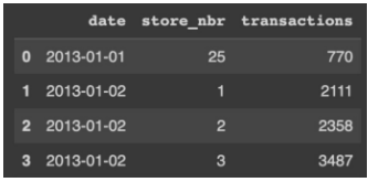
Figure 2: Sales dataset preview
After loading the data in redshift or any other SQL engine supported by DBT, we have to set it up to connect to our database. Here is a link to the official documentation to learn how to do it.
Once the link between DBT cloud and the database engine is configured the workspace status in the right bottom corner will be green and we can start running queries.

Figure 3: DBT: Ready-to-Execute Queries
Setting up the project
The project tree could be generated automatically within the DBT interface. The generated project has the following tree structure. All our queries will be stored in the models folder**.**
For this article, you can find my git repository here with the queries that we will see below.
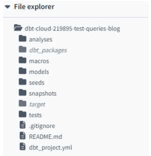
Figure 4: DBT Project Structure
Although it is not compulsory, it is very recommended to fill the schema.yml file within the models folder. Actually, defining tables structures in schema.yml in dbt serves several important purposes:
-
Documentation: The schema.yml file serves as a form of documentation. It provides a clear and centralized place for you and your team to document the structure of dbt models. This documentation is often used to generate data dictionaries.
-
Testing: The tests section in the schema.yml file allows you to define data tests for each column. These tests can include checks for null values, uniqueness, and other data quality checks.
-
Consistency: By defining the table structure in schema.yml, we can ensure that the structure of our dbt models aligns with our expectations. This can be especially important when working in a team where multiple people might be contributing to the dbt project.
Therefore, even if the table exists and is documented in the database, defining it in the schema file with details is recommended. Here is how we could define it.
Running the first query
Each query or table transformation in DBT is stored in a separate .sql file inside a models folder. In order to test our setup we can create a sales.sql file and run
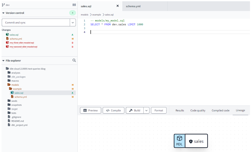
Figure 5: DBT interface showing project structure and lineage
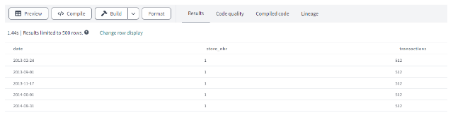
Figure 6: Sales data preview in DBT
Notice that the tab preview and lineage got populated.
Now that the project and the first table is set up, we will be able in the next section to try different queries to build new features.
**Example 1 - Basic Aggregation
**
Coming back to our sales data, a feature that we can generate could be based on operations like AVG, SUM that we can use within an SQL query. Here is an example to compute the total sales by store.
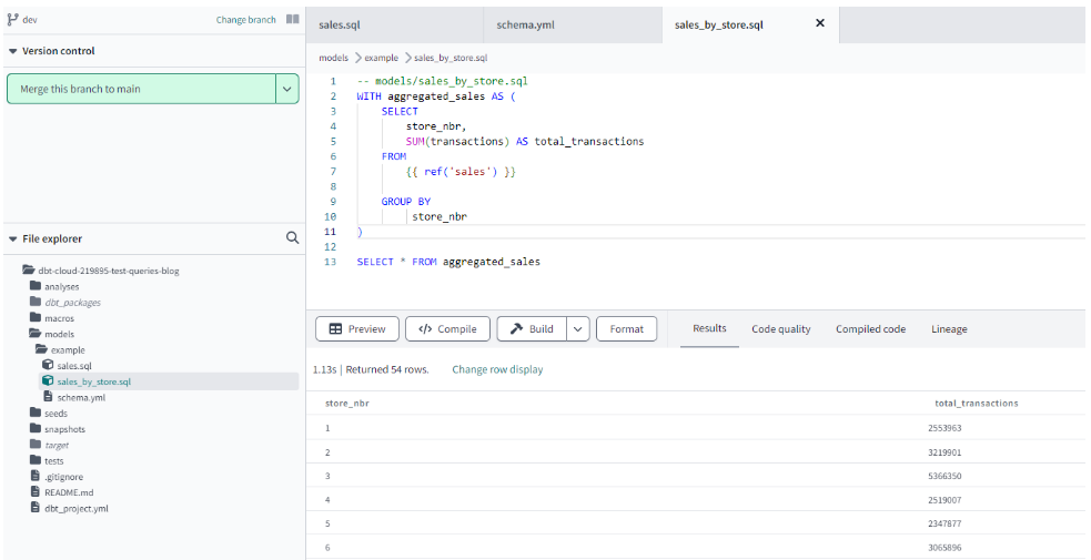
Figure 7: Total sales by store transformed data
Notice here that we use {{ ref('sales') }}, this ref function tells DBT to interpret "sales" as a model. Also, when looking at lineage we can observe that we are starting to have DAGs to describe links between models. This feature is useful both for us when we start getting complex workflows and is used by DBT internally to compute the tables and manage their dependencies correctly. Here’s how the lineage looks like now:
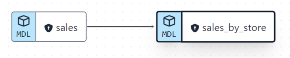
Figure 8: DBT Lineage showing the sales by store data as a direct transformation of sales
**Example 2 - Window Functions
**
Window functions in SQL are used to perform calculations across a specified range of rows related to the current row. As an example, we will create the Total sales per store using window functions. So that in each row, we get the total sales over the whole period. Such a metric could be used as a feature to highlight the store’s activity when dealing with time series data. We can use the OVER clause along with the PARTITION BY clause to group the data by store. Here is an example.
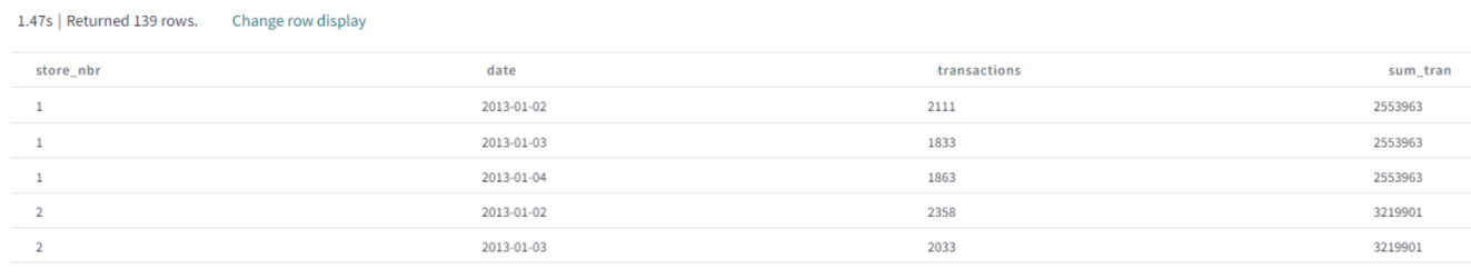
Figure 9: Sales by store x data query results
So, in this query we used the window function to compute the SUM of sales on the whole dataset period and propagate it to all the available dates. As expected we obtain the same value of total sales by store. The difference between the group by and window is that the former aggregates the rows to get one row per designated group by keys, however the latter keeps the same dataset number of rows and propagates the value over all the rows sharing the same PARTITION BY key. Now if we look at our project lineage we can see that a new link has appeared.
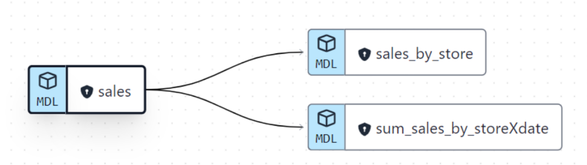
Figure 10: DBT Lineage showing the last two queries transformations
**Example 3 - Joining and Data Merging
**
The Lineage above shows how the two models that have been created are resulting from a transformation of the sales model. The same logic applies when we build a table that is based on two sources, let’s take an example of a join operation:
In the first query we aggregated the date at the store level to have the total sales by store.
- In the second one, we used the window function to compute the sum of transactions by store and project its value at daily level.
- A common column between the two tables is the store_nbr. Now let’s try to join those two tables on the store_nbr. This query should give us a dataset at daily x store level with two columns sum_sales_groupby, sum_sales_window. Both should have the same values as we are showing two calculation methods to achieve the same result.
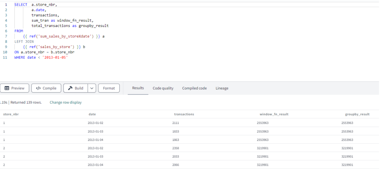
Figure 11: DBT model and data preview
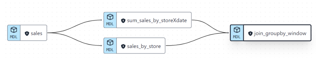
Figure 12: DBT lineage showing the last join operation
Example 4 - Using Lag Function
Here our goal is to use the Lag function in SQL to compute a metric. An example of a feature, could be the sales of last week. So, for each store at each date we would like to report the sales or transactions of last week. We can achieve this by using a lag function to shift rows. Yet, as we have multiple stores in the dataset, the query should consider the store_nbr column so that data for different stores don’t mix. To achieve this we use the Lag combined with a window function.
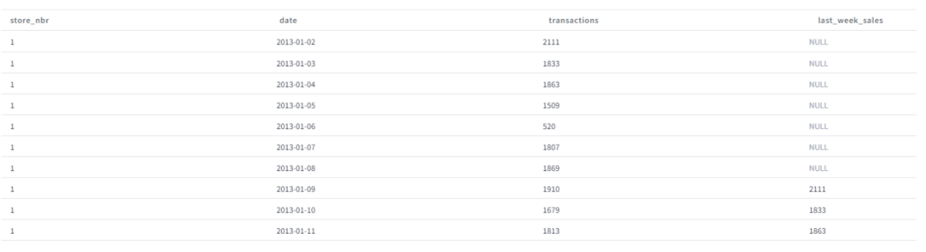
Figure 13: Example of the lag transformation results (store 1)
The pattern is repeated for each store. You can notice that for each store the first 7 rows have null values as no data is available before the first dates, then we start observing the sales from last week. Same behavior is observed for all stores.
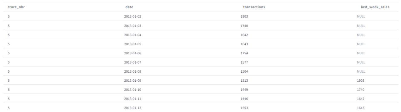
Figure 14: Example of the lag transformation results (store 5)
This is how our lineage looks like now:
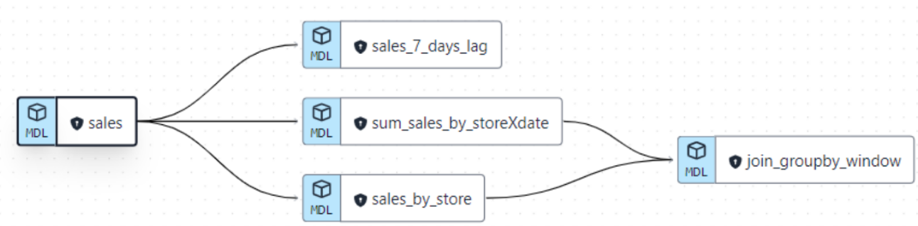
Figure 15: DBT lineage showing the link between the different implemented models
Example 5 - Combining Aggregation, Window and Lag functions in a Real Scenario
Now that we have seen different functions to create features in sql using aggregations, window and lag functions, we can imagine working on a pipeline to prepare data for a time series forecasting model that would forecast short term demand. The data we have at hand is the one used in this previous section giving daily sales by store.
For our forecasting model, we will, for sake of simplicity, use 3 features:
- Total sales for the store as an indicator of activity (model can learn for instance whether it’s a big or small store).
- 7 days Lag of sales in a given store as an indicator of sales on the same day of last week. Time varying features are always important when forecasting sales. In real world scenarios we often use multiple lags.
7 days sales moving average. Moving averages give a smoothed value that can reflect a short term trend and help a machine learning model learn.
As the first two were already created in example 2 and 4, here is the query for the last feature:
Finally, in order to join the different tables and build the final dataset, we can create a new .sql file with the following join query:
Here is how our final dataset looks like, our joined_sales_data table is now ready.
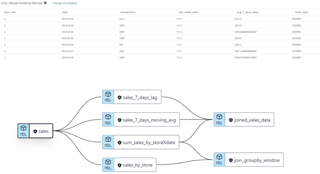
Figure 16: Results of the different implemented queries and their relationships
You can notice that the modular design allows us to break down complex data transformations into smaller, manageable units, or "models," which can be developed and tested independently. This modularity enhances collaboration and parallel development efforts within a team.
Furthermore, DBT's version-controlled approach, often integrated with tools like Git, enables tracking changes to the data models over time. This not only facilitates versioning for auditing and reproducibility but also streamlines collaboration by providing a clear history of modifications.
In addition to that, DBT offers a seamless way to generate documentation for such workflows.
Here are more details on how to generate and serve it. The documentation pipeline uses the lineage and the content of the schema.yml file to generate well structured html pages in which we can see models, columns names,types and description.
Summary
In this article, we've explored the practical applications of DBT for a data warehouse in constructing feature engineering pipelines. We've demonstrated the value of adopting a modular approach to constructing datasets, promoting clarity and ease of maintenance over lengthy SQL queries. This not only makes the process easy but also opens up new perspectives for efficient and scalable feature engineering practices.